|
|
In this chapter, we show the performance results of scheduling workflow applications on a simulated grid environment using the GRACCE scheduling algorithms.
The GRACCE workflow scheduler targets computational grid environments that comprise parallel computing resources owned by different organizations. But there are difficulties in evaluating a workflow scheduler in a real grid environment. These include the limited number of resources available for testing purpose, and the impossibility of creating a repeatable and traceable environment for evaluating different scheduling strategies under different resource loads. For these reasons, we perform our experiments in a simulated grid environment that models a real grid very closely in those respects that are important for workflow scheduling. The experimental environment consists of simulated grid resources with a variety of computational capabilities and different network bandwidth between resources, simulated grid jobs and the local schedulers of resources, and a random job generator that models the resource users. We have also developed a random workflow generator that is able to create workflows with different task specifications and dependency relationships for evaluating our scheduling methods.
In our simulation, a resource is configured with a total number of PEs and a total number of MIPS (Million Instructions Per Second) to represent its computational capability, an approach borrowed from the GridSim toolkit [104]. GridSim has limitations in its manner of scheduling parallel applications, and thus cannot be directly exploited for our work. In GridSim, a parallel job that requires more than one PE is normalized to a single-PE job (Gridlet in GridSim term). When a job requests 10 PEs and 15 minutes execution time, GridSim allocates one PE and sets the execution time to 10*15 minutes. For this reason, we have developed our own local scheduler for the simulated resources. It allows us to allocate or reserve multiple PEs for a parallel job, and it keeps track of currently used PEs (and thus the available PEs) in order to serve other requests.
The scheduling policy of the local scheduler is first-come-first-serve (FCFS) space-sharing with resource advanced reservation. The scheduler maintains a job queue for the resource, and a newly submitted job is put at the tail of the queue. The local scheduler allocates PEs for the job at the head of the queue when another job completes its execution and releases the PEs. If there are not enough available PEs for the job at the head of the queue, the job (and all those behind it) has to wait until another job completes and releases enough PEs. If an advanced reservation is used when submitting a job, the job does not need to wait and is launched when the reservation becomes active. So we basically implement a gang scheduling policy [105] that is widely used for parallel application scheduling.
The simulated grid consists of eight resources. Their configurations are shown in Table 7.1. The MIPS per PE (MIPS/PE) is calculated to represent the computation speed of the resource’s PEs. The greater the MIPS/PE, the faster the resource. The network bandwidth between every pair of resources in the simulation is calculated by generating a random bandwidth between the minimum bandwidth (0 MB/s) and the maximum bandwidth (10 MB/s).
|
A grid job (or a workflow task) in our simulation environment requests resources in terms of the total number of instructions (in the unit of Millions Instructions (MIs)), and the number of PEs. We assume that the instructions are evenly distributed and executed on the PEs, thus we have the parameter of MIs/PE for a job. In this modeling schema, the base execution time (bExeTime) of a job on a resource is equal to the job’s MIs/PE divided by the resource’s MIPS/PE. The base execution time is the ideal execution time of the job on the resource without considering the impacts of those factors, such as cache misses, or disk accesses that may stall the CPU calculation. We call those factors non-CPU factors with regard to their impacts on the job’s performance.
A job execution is simulated using a timer thread: when the thread starts, the job starts; when it times out, the job completes. The timeout interval of the thread, corresponding to the execution time (ExeTime) of the job, is calculated by adding an additional time to the bExeTime that represents the impact of those non-CPU factors on the job execution. To simplify our simulation, this additional execution time (aExeTime) is modeled as bExeTime * Random (0, extFactor), where extFactor is a number between 0.0 and 1.0 representing the impacts of these factors. The Random (0, extFactor) is a random number between 0 and extFactor.
In this schema, the job execution time includes both the CPU time and the time for memory and disk/network accesses, thus closely models a real job execution on a real computational resource. Furthermore, we can easily define a schema for estimating the execution time of the job on a resource by using one property of the Random(0, extFactor) function: the arithmetic mean of an infinite number of numbers generated by Random(0, executor) is equal to exeFactor / 2. So the estimated execution time (eExeTime) can be modeled as bExeTime * (1 + exeFactor / 2). In this way, the estimated execution time equals the real execution time statistically; and the difference between Random(0, extFactor) and exeFactor / 2 introduces the unpredictable part of the execution time. We formulate the two schemas as follows:
ExeTime = bExeTime * (1 + Random(0, extFactor))
eExeTime = bExeTime * (1 + extFactor / 2)
To mimic grid resource users, we have created a random job generator that creates and submits jobs with different resource requirements to the local scheduler of a resource. The job generator is able to maintain the average resource load at a specific value between 0.0 and 1.0. The resource load at a given time is calculated by dividing the number of occupied PEs by the total number PEs of the resource. If the current resource load is less than the expected load, the job generator creates and submits jobs; otherwise it waits and monitors the resource load. As a multi-threaded program, the job generator is independent of the resource simulator, the local scheduler and the workflow scheduler. It, hence, models the multiple users of the resources.
We have also created a random workflow generator to create different workflows for evaluating workflow scheduling algorithms. The workflow generator creates workflow tasks as the grid jobs, and then creates the dependency relationships between these tasks and sets the size of the intermediate files between the dependent tasks. The task specifications and dependency relationships, such as the number of PEs and the MIs, the number of parent and child tasks, and the intermediate file sizes between its parent/child tasks, are all controllable. The generator gives users options to specify the maximum and minimum of a parameter, and uses the Random(min, max) operation to generate a random value for the parameter. The number of tasks allowed in the generator is 0 to 200. A generated workflow can be simply visualized using yFiles graph library [106].
The performance of a workflow execution is measured by the time to complete the execution, i.e., from the time when users submit a workflow to the time that the results are produced. The execution of a workflow involves both the execution of the workflow tasks and the transfer of immediate files between dependent tasks. The execution time is not simply the sum of the times for task execution and for the file transfers. Some executions and/or transfers may be overlapped, and additional times may be introduced due to the unavailability of resources for ready tasks. As a result, the total workflow execution time consists mainly of three parts: the task execution time, data transfer time and the time spent waiting for resources to be available.
Obviously, the task execution time is not simply the sum of times spent carrying out all tasks because some of them are executed concurrently. For a workflow that can be modeled as a DAG, critical tasks are those that must be started on their earliest start times in order to achieve the best performance of the workflow execution. The sum of the execution times of critical tasks is the time spent for workflow task execution. So if we know the critical tasks of a workflow, we can easily calculate its task execution time. Yet during the workflow execution, the critical path is changing because the time spent on a task execution is not fixed. This is the issue of dynamic critical path. In our scheduler, an initial critical path is calculated based on the estimated task execution time. During workflow execution, the scheduler compares the subworkflow of completed tasks with the subworkflow of uncompleted tasks and adjusts the critical path so that it matches with the real execution pattern.
The time spent executing a task depends on what resource is allocated for it. In general, a workflow scheduler searches for the fastest available resource for a task. So in a computational grid, the overall grid load impacts the choice of resource. The higher the load is, the more likely a slower resource is allocated for the task. But if the workflow scheduler is able to reserve resources for a task in advance, a fast resource can be allocated even in a high-load environment.
The workflow scheduler, working on top of the local schedulers of grid resources, cannot launch a workflow task on the allocated resource directly. It has to submit it in the form of a job to the local scheduler, which schedules the job based on its own policies. This local scheduler may queue the job for any reason, for example, if the resource is heavily loaded or higher-priority jobs come in and have to be scheduled earlier. So even when a task is ready, it may be queued by the local scheduler. The time period from when the task is ready to when it is launched by the local scheduler is often referred to as the “queue waiting time”.
For a task that is submitted to the local scheduler, the length of queue waiting time depends on many factors, including the resource load, the number of CPUs requested by the job, the characteristics of the jobs currently running and those queued in the local scheduler, and the scheduling policies applied. It is difficult to predict [107]; there have been several efforts [108, 109, 110] to develop prediction mechanisms in the local schedulers. In general, the higher the resource load is, the longer the queue waiting will be. Again, if a task is submitted to a resource that has been reserved in advance, the queue waiting time can be greatly reduced.
In our simulation environment, as long as we know the allocated resource for a task, the execution time can be easily predicted, i.e., the eExeTime calculated using the formula in the last section. Also, since we use the FCFS space-sharing scheduling policy with advanced reservation, we can estimate the start time for a newly submitted job by performing a simulated execution of current running jobs and the queued jobs, a process that sums up the estimated execution time of the tasks that occupy the majority period of the resource while considering the advanced reservation created for the resource. We can then calculate the queue waiting time easily. In our workflow scheduler, this prediction schema is used when planning the workflow execution. Lastly, we want to note that the queue waiting for a non-critical task does not delay the overall workflow execution if it does not delay the launching of critical tasks.
If the parent task and child task in a data dependency relationship are allocated on different resources, intermediate files need to be transferred between the two resources. If the network is slow and the intermediate files are large, the data transfer time may become a significant part of the overall workflow execution time. But at run time, file transfers are overlapped with the execution of tasks. So not all data transfers impact the workflow performance; only those that delay the launching of critical tasks, directly or indirectly, do so.
Using the simulation environment and the resource local scheduler we have developed, we have implemented two workflow schedulers based on the algorithms we discussed in the last chapter: the just-in-time workflow scheduler that is widely used in most of current workflow systems, and the GRACCE scheduler with full workflow planning and resource reservation policy. Using the just-in-time scheduler, when the parent tasks of a task are completed, the scheduler allocates a resource for it, and then submits it the local scheduler of the allocated resource. In the GRACCE workflow scheduler, the execution of the workflow is planned in advance before it is launched. Resources are allocated and reserved for the workflow tasks during the planning process. The GRACCE scheduler launches each workflow task according to the planned schedule for the task. Both of the two schedulers take into account the time spent to transfer immediate data file between the parent task and the child task when allocating a resource for the child task. In the rest of this section, we evaluate the performance of the workflow execution using the two schedulers in our simulated grid environment. The assumptions made in using the two schedulers and in discussing the performance results are as follows:
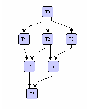
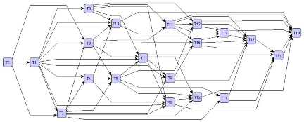
Our first workflow example is a 7-task workflow, as shown in Figure 7.1, and the task specifications and dependency specifications are shown in Table 7.2 and Table 7.3.
|
|
Under our grid simulation environment, both of the two schedulers can easily find the optimal schedule for the workflow in Figure 7.1 and using this schedule, the best performance can be achieved. This schedule is made under the assumption that all the grid resources are available for the workflow, i.e., the resource load is 0 and the network bandwidth is the maximum one (10 MB/s). There is no queue waiting when submit a task to the local scheduler. The optimal schedule for the 7-task workflow is shown in Table 7.4. In this schedule, the critical tasks are T0, T2, T5, T76. Of the workflow execution, the total time spent for executing tasks, i.e., 344.4 seconds, is the sum of the execution times of the critical tasks; the executions of non-critical tasks overlap the executions of critical tasks. The total time spent for transferring immediate files, i.e., 110 seconds, is the sum of the transfer times for the input files to the critical tasks, while considering the overlapping transfers of multiple files to the same task.
| |||||||||||||||||||||||||||||||||||||||||||||||||||||||||||||||||||||||||||||||||||||||||||||||||||||||||||||||||||||||||||||||||||||||||||||||||||
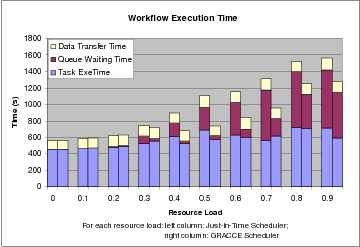
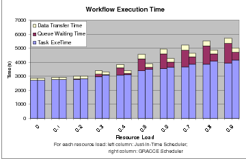
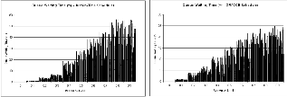
Figure 7.2 shows the execution time of the 7-task workflow under resource load from 0.0 to 0.9 using the just-in-time scheduler and the GRACCE scheduler. The workflow execution time increases as the load of grid resources increases. But under the same resource load, the GRACCE scheduler achieves a significant reduction in execution time compared to the just-in-time scheduler. The biggest difference is the queue waiting time in the two schedulers. The data transfer time and the task execution time do not change a lot as the resource load changes.
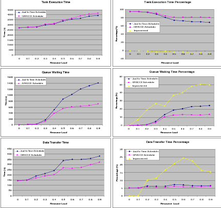
The distribution of the workflow execution time is shown in Figure 7.3. The time spent in task execution increases generally as the resource load increases, but not uniformly. The scheduler does not necessarily allocate the fastest resource available for a workflow task. The two schedulers consider both the queue waiting time and the time to transfer the intermediate files when allocating a resource. The GRACCE scheduler also takes into account whether an advanced reservation has been granted. So it is very common that the scheduler allocates a slower resource to a task, either because it has been reserved or because it leads to a shorter queue waiting time.
When the resource load is above 0.2, the queue waiting time is reduced greatly under the GRACCE scheduler. Although the queue waiting time increases when the resource load rises above 0.3 under both schedulers, the savings achieved using the GRACCE scheduler are significant, from 35% to 85%. The reason why the GRACCE scheduler cannot cut down the queue waiting time to the minimum under higher resource load is because most of these queue waiting times are spent by the first several tasks, and it is too late to reserve a resource without introducing any queue waiting.
Similar to the task execution time, the data transfer time does not change a lot under different resource loads. That is because the data transfers for the same level of tasks, such as T1, T2 and T3, or T4 and T5, or T6 are overlapped, and of the total 7 tasks, such three overlapped transfers do not introduce much of the performance increase or decrease in the overall workflow execution time. In terms of the data transfer time percentage, it is similar to the task execution time percentage. They both decrease as the resource load increases, which is mainly because the total workflow execution time increases greatly.
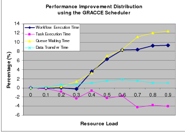
In Figure 7.4, we show the distribution of the improvement obtained for the 7-task workflow by using the GRACCE workflow scheduler rather than the just-in-time scheduler. The performance improvements come mostly from the reduction in queue waiting time. We can also see from the figure that the biggest improvement comes when the resource load is 0.5. Before this point, the minimum queue waiting time is reached. With resource load above 0.5, even the GRACCE scheduler cannot reduce the queue waiting time to the minimum because it is too late to make immediate resource reservation for the first several tasks under higher resource load. That is why we cannot see the similar performance improvement under higher resource load.
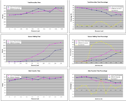
We next consider a 20-task workflow, shown in Figure 7.5. It has much higher MIs for each task than in the 7-task workflow, which means that the task execution time is a more significant contributor to the workflow execution. The workflow execution times under the two schedulers are plotted in Figure 7.6. It shows that the workflow execution time using the GRACCE scheduler is less than that using the just-in-time scheduler when the resource load is above 0.3. The same as the 7-task workflow execution, most of the reduction in execution time comes from the lower queue waiting time.
The Figure 7.7 shows the distribution of the workflow execution time and the percentage of each individual processing time in the total workflow execution time using the two schedulers. The task execution time using the GRACCE scheduler is greater than that using the just-in-time scheduler when the resource load is above 0.1. We have mentioned the reason before when we evaluated the 7-task workflow. In terms of the queue waiting time, we see the GRACCE scheduler is able to reduce it greatly when the resource load is above 0.4. For the data transfer time, using the GRACCE scheduler improves by about 10% to 25% with resource load above 0.2. But using both schedulers, the data transfer time is only a very small portion of the workflow execution, about 5%, so the performance improvement using the GRACCE scheduler does not substantially reduce the overall execution time.
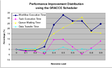
The distribution of performance improvement under the GRACCE scheduler is shown in Figure 7.8. For a moderate to high resource load (0.4 to 0.9), the GRACCE scheduler is able to reduce the workflow execution time by about 4% to 9%, the queue waiting time by about 4% to 12% and data transfer time by about 1% to 2%. However, it slows down the workflow task execution by 2% to 5%. As for the 7-task workflow, the reduction of queue waiting time contributes most of the performance improvement of the workflow execution.
In order to compare the performance obtained under the two scheduling approaches, we have collected the execution times of 60 workflows that were generated by our random workflow generators. The queue waiting time percentages in the total workflow execution times of these workflows using the two schedulers are plotted in Figure 7.9. Using the just-in-time scheduler, the queue waiting time is in the range of 0% to 55%. If using the GRACCE scheduler, the range is of 0% to 25%. So our GRACCE scheduler with workflow planning and reservation is able to reduce the queue waiting time significantly under different resource loads.
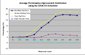
The average performance improvement distribution obtained by using the GRACCE scheduler is shown in Figure 7.10. The workflow execution time is reduced from 2% to 20% if the resource load is above 0.3. As in our examples, the reduction of queue waiting time is the biggest contributor. Again the reduction of data transfer time is within 3% and the task execution time increases by about 3% to 5%. We can also see that the biggest performance improvement is obtained with a load of 0.6 to 0.7.
In summary, compared to the widely-used just-in-time scheduler, our GRACCE scheduler is able to improve the workflow execution performance by about 20% under moderate and high resource load. This performance improvement is achieved by the reduction of the task queue waiting time using the techniques of workflow execution planning and resource advanced reservation. In order to reduce the overall queue waiting time, the scheduler may allocate slower resources to some workflow tasks, causing the increase of the task execution time.